Introduction
After a new policy is enacted, we often want to estimate what effects the policy had. Difference-in-differences (diff-in-diff) is one way to estimate the effects of new policies. To use diff-in-diff, we need observed outcomes of people who were exposed to the intervention (treated) and people not exposed to the intervention (control), both before and after the intervention. For example, suppose California (treated) enacts a new health care law designed to lower health care spending, but neighboring Nevada (control) does not. We can estimate the effect of the new law by comparing how the health care spending in these two states changes before and after its implementation.
Thanks to its apparent simplicity, diff-in-diff can be mistaken for a “quick and easy” way to answer causal questions. However, as we peer under the hood of diff-in-diff and illuminate its inner workings, we see that the reality is more complex.
Notation
The table below provides a guide to the notation we use throughout this site.
| Symbol | Meaning |
|---|---|
| \(Y(t)\) | Observed outcome at time \(t\) |
| \(A=0\) | Control |
| \(A=1\) | Treated |
| \(t=1,\ldots,T_0\) | Pre-treatment times |
| \(t=T_0+1,\ldots,T\) | Post-treatment times |
| \(Y^a(t)\) | Potential outcome with treatment \(A = a\) at time \(t\) |
| \(X\) | Observed covariates |
| \(U\) | Unobserved covariates |
Target estimand
At the outset of any analysis, we first define a study question, such as “Did the new California law actually reduce health care spending?” This particular question is aimed at determining causality. That is, we want to know whether the new law caused spending to go down, not whether spending went down for other reasons.
Next, we transform our question into a statistical quantity called a target estimand. The target estimand, or target parameter, is a statistical representation of our policy question. For example, the target estimand might be “the average difference in health care spending in California after the new law minus average health care spending in California if the law had not been passed.” This target estimand is written in terms of potential outcomes. In our toy scenario, California has two potential outcomes: health care spending under the new law and health care spending without the new law. Only one of these is observable (spending with the new law); the other is unobservable because it didn’t happen (spending without the new law).
Third, we choose an estimator, which is an algorithm that uses data to help us learn about the target estimand. Here, we focus on the diff-in-diff estimator, which relies on some strong assumptions, including that health care spending in Nevada can help us understand what would have happened in California without the new law. That’s how we can use observed data to learn about a target estimand that is written in terms of unobservable outcomes. More on this later.
With all these elements in place, now we can actually compute our estimate, a value of the estimand found by applying the estimator to the observed data.
To recap,
The quantity we care about is called the estimand. We choose a target estimand that corresponds to our policy question and express it in terms of potential outcomes.
The algorithm that takes data as input and produces a value of the estimand is called the estimator.
The estimator’s output, given data input, is called the estimate. This value represents our best guess at the estimand, given the data we have.
![]()
As noted above, we define the target estimand in terms of potential outcomes. In the California example, we used the average effect of treatment on the treated (ATT). This compares the potential outcomes with treatment to the potential outcomes with no treatment, in the treated group. For a diff-in-diff, the ATT is the effect of treatment on the treated group in the post-treatment period. Written mathematically, the ATT is
Average effect of treatment on the treated (ATT) \[\begin{equation*} ATT \equiv \mathbb{E}\left[Y^1(2) - Y^0(2) \mid A = 1\right] \end{equation*}\]
Recall that \(Y^a(t)\) is the potential outcome given treatment \(a\) at time \(t\). Here, \(t = 2\) represents the post-treatment period, \(a = 1\) represents treatment and \(a = 0\) represents no treatment. Translated literally, the equation is \[\begin{equation*} \mbox{Expected}\left[\mbox{Spending in CA with the new law} - \mbox{Spending in CA without the new law}\right] \end{equation*}\]
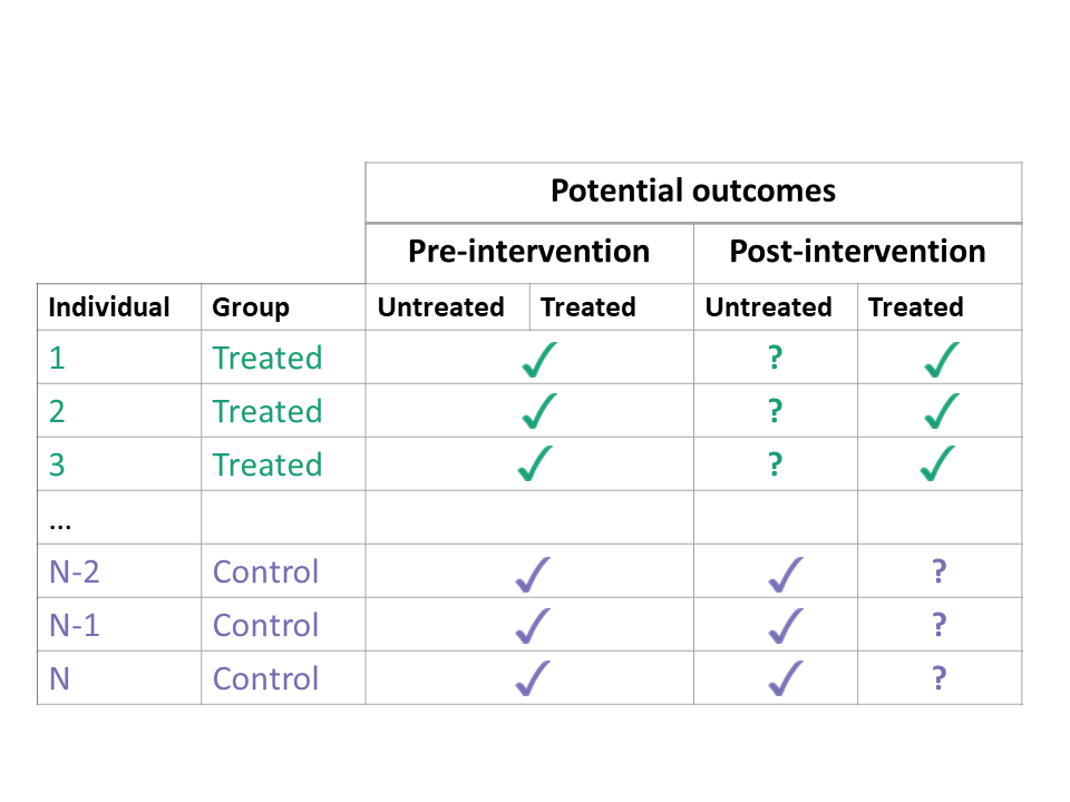
If we could observe the potential outcomes both with treatment and with no treatment, estimating the ATT would be easy. We would simply calculate the difference in these two potential outcomes for each treated unit, and take the average. However, we can never observe both potential outcomes at the same time. In the treated group, the potential outcomes with treatment are factual (we can observe them), but the potential outcomes with no treatment are counterfactual (we cannot observe them).
So how do we estimate the ATT when the some of the potential outcomes are unobservable? In diff-in-diff, we use data from the control group to impute untreated outcomes in the treated group. This is the “secret sauce” of diff-in-diff. Using the control group helps us learn something about the unobservable counterfactual outcomes of the treated group. However, it requires us to make some strong assumptions. Next, we discuss assumptions required for diff-in-diff.
Assumptions
Consistency
For diff-in-diff, the treatment status of a unit can vary over time. However, we only permit two treatment histories: never treated (the control group) and treated in the post-intervention period only (the treated group). Thus, we will use \(A=0\) and \(A=1\) to represent the control and treated groups, with the understanding that the treated group only receives treatment whenever \(t > T_0\) (see notation).
Every unit has two potential outcomes, but we only observe one — the one corresponding to their actual treatment status. The consistency assumption links the potential outcomes \(Y^a(t)\) at time \(t\) with treatment \(a\) to the observed outcomes \(Y(t)\).
Consistency Assumption
\[
Y(t) = (1 - A) \cdot Y^0(t) + A \cdot Y^1(t)
\]
If a unit is treated \((A=1)\), then the observed outcome is the potential outcome with treatment \(Y(t) = Y^1(t)\) and the potential outcome with no treatment \(Y^0(t)\) is unobserved. If a unit is not treated \((A=0)\), then \(Y(t) = Y^0(t)\) and \(Y^1(t)\) is unobserved.
However, we also assume that future treatment does not affect past outcomes. Thus, in the pre-intervention period, the potential outcome with (future) treatment and the potential outcome with no (future) treatment are the same. We write this assumption mathematically asArrow of time \[ Y(t) = Y^0(t) = Y^1(t),\; \mbox{for}\ t \leq T_0 \]
For recent work that relaxes the consistency assumption, see Wang (2023). Wang (2023) considers a panel data setting with interference over both space and time. This means that any individual unit’s potential outcome at a particular time period can depend not only on a unit’s individual assignment, but also on the treatment status of all units over all time periods. Therefore, each unit in each time period may have more than only two potential outcomes. In this setting, Wang (2023) defines the marginalized individualistic potential outcome, i.e., the average of all potential outcomes for unit \(i\) at time \(t\) (holding fixed the treatment history of unit \(i\) up to time period \(t\)) corresponding to all the ways other units could be treated or untreated over all time periods. The marginalized individualistic treatment effect is simply a contrast between the marginalized individualistic potential outcomes of two treatment histories, and the overall marginalized average effect (AME) for the contrast of any two treatment histories is simply the average of the marginalized individualistic treatment effects. In practice, Wang (2023) also makes the assumption that future treatment does not affect past outcomes, which reduces the number of potential outcomes for each unit under a particular treatment history. This assumption, along with a particular “ignorability” condition facilitates estimation and inference, both of which roughly adhere to the treatments in the Estimation and Inference sections below.
Counterfactual assumption (Parallel Trends)
A second key assumption we make is that the change in outcomes from pre- to post-intervention in the control group is a good proxy for the counterfactual change in untreated potential outcomes in the treated group. When we observe the treated and control units only once before treatment \((t=1)\) and once after treatment \((t=2)\), we write this as:
Counterfactual Assumption (1) \[\begin{align*} \mathbb{E}\left[Y^0(2) - Y^0(1) \mid A = 1\right] = \\ \nonumber \mathbb{E}\left[Y^0(2) - Y^0(1) \mid A = 0\right] \end{align*}\]
This is an assumption — not something we can test — because it involves unobserved counterfactual outcomes, namely \(Y^0(2)\) for \(A = 1\).
In the shiny app embedded below, we can see what the counterfactual assumption does and how we calculate the ATT under our assumptions. The solid black lines represent the observed data. When we click the “Impute Counterfactual from Control to Treated” button, the slope of the line of the control group is imputed to the treated group (dashed line). Finally, clicking the “Show diff-in-diff effect button” reveals how we calculate the average effect of treatment on the treated (ATT).
Traditionally, this assumption is called the parallel trends assumption, but as we will soon see, that term can be ambiguous.
Positivity Assumption
Lastly, we make a positivity assumption. With the positivity assumption, we assume that treatment is not determinant for specific values of \(X\). Thus, for any \(X = x\), the probability of being treated (or untreated) lies between 0 and 1, not inclusive.
Positivity Assumption \[\begin{equation*} 0 < P(A = 1 | X) < 1 \; \text{ for all } X. \end{equation*}\]
We will invoke the positivity assumption explicitly when we discuss semiparametric and nonparametric estimators.
Identification
Using the assumptions above, we can re-write the target estimand (which involved unobserved counterfactuals) in a form that depends only on observed outcomes. This process is called “identification”.
For diff-in-diff, identification begins with the ATT, applies the Counterfactual Assumption (1) and the Consistency Assumption, and ends with the familiar diff-in-diff estimator.
The result is the familiar diff-in-diff estimator
\[\begin{align*} ATT &\equiv \mathbb{E}\left[Y^1(2) - Y^0(2) \mid A = 1\right] \\ &= \lbrace \mathbb{E}\left[Y(2) \mid A = 1\right] - \mathbb{E}\left[Y(1) \mid A = 1\right] \rbrace - \\ & \ \ \ \ \ \ \lbrace \mathbb{E}\left[Y(2) \mid A = 0\right] - \mathbb{E}\left[Y(1) \mid A = 0\right] \rbrace \end{align*}\]
For a straightforward estimate of the ATT, we could simply plug in the sample averages for the four expectations on the right-hand side:
- The post-intervention average of the treated group for \(\mathbb{E}\left[Y(2) \mid A = 1\right]\);
- The pre-intervention average of the treated group for \(\mathbb{E}\left[Y(1) \mid A = 1\right]\);
- The post-intervention average of the control group for \(\mathbb{E}\left[Y(2) \mid A = 0\right]\);
- The pre-intervention average of the control group for \(\mathbb{E}\left[Y(1) \mid A = 0\right]\).
Finding the standard error for this estimator is a little more complex, but we could estimate it by bootstrapping, for example.
Sometimes the counterfactual assumption may hold only after conditioning on some observed covariates, and the identification becomes more complex. More on this in the Confounding section.
Multiple time periods
When we observe the treated and control units multiple times before and after treatment, we must adapt the target estimand and identifying assumptions accordingly. Let’s start by looking at possible target estimands.
Target Estimands
We can calculate the ATT at any of the post-treatment time points
Time-varying ATT
at each time point
For some \(t > T_0\),
\[\begin{equation*}
ATT(t) \equiv \mathbb{E}\left[Y^1(t) - Y^0(t) \mid A = 1\right]
\end{equation*}\]
or we can compute the average ATT across the post-treatment time points
Averaged ATT
over all time points
\[\begin{equation*}
ATT \equiv \mathbb{E}\left[\overline{Y^1}_{\{t>T_0\}} - \overline{Y^0}_{\{t>T_0\}} \mid A = 1\right]
\end{equation*}\]
Here, the overbar \(\overline{{\color{white} Y}}\) indicates averaging and the subscript \(_{\{t>T_0\}}\) refers to the time points over which the outcome is averaged.
The above estimands make sense when the treatment is administered at the same time for all treated groups. When treatment timing differences occur, Athey and Imbens (2022) and Goodman-Bacon (2021) discuss the weighted estimands that arise. We discuss diff-in-diff when there is variation in treatment timing briefly in the estimation section.
Assumptions for Multiple Time Points
What kind of assumptions do we need to estimate the ATTs above? We consider several counterfactual assumptions that may require:
- parallel average outcomes in pre- to post-intervention periods
- parallel outcome trends across certain time points, or
- parallel outcome trends across all time points.
First, consider an assumption that averages over the pre- and post-intervention time points, effectively collapsing back to the simple two-period case.
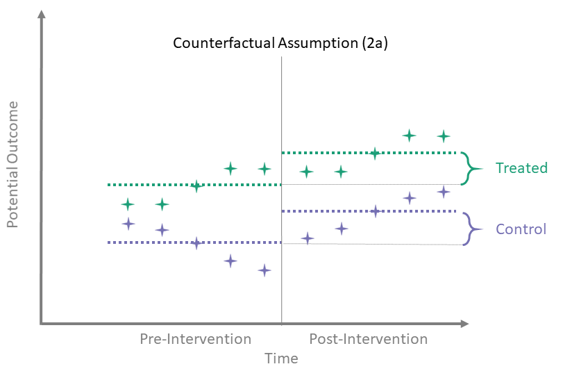
Counterfactual Assumption (2a)
Avg pre, avg post
\[\begin{align*}
\mathbb{E} \left[\overline{Y^0}_{\{t > T_0\}} - \overline{Y^0}_{\{t \leq T_0\}} \mid A = 0\right] = \\
\mathbb{E} \left[\overline{Y^0}_{\{t > T_0\}} - \overline{Y^0}_{\{t \leq T_0\}} \mid A = 1\right]
\end{align*}\]
Here, we assume that the difference between the average of the pre-intervention outcomes and the average of the untreated post-intervention outcomes is the same for both treated and control groups. To identify the time-averaged ATT using this assumption, we use the same identification process as in the simple case with only one observation in each of the pre- and post-intervention periods.
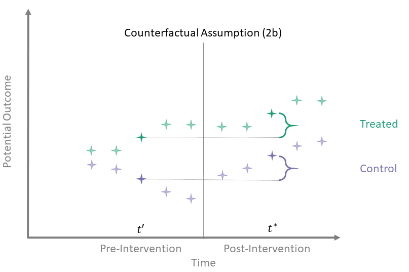
Counterfactual Assumption (2b)
One pre, one post
For some \(t^* > T_0\), there exists a \(t' \leq T_0\) such that
\[\begin{align*}
\mathbb{E}\left[Y^0(t^*) - Y^0(t') \mid A = 1\right] = \\
\mathbb{E}\left[Y^0(t^*) - Y^0(t') \mid A = 0\right]
\end{align*}\]
Counterfactual Assumption (2b) essentially disregards time points other than these two. That is, the other time points need not satisfy any “parallel trends” assumption. While this assumption is perfectly valid if true, using such an assumption requires justification. For instance, why do we believe this assumption is satisfied for two time points but not the rest? To identify the ATT using this assumption, we again use the same identification process as in the simple case, since we are back to considering only one time point pre-intervention and one time point post-intervention.
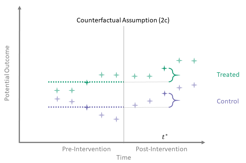
Counterfactual Assumption (2c)
Avg pre, one post
For some post-treatment time point \(t^* > T_0\),
\[\begin{align*}
\mathbb{E}\left[Y^0(t^*) - \overline{Y^0}_{\{t \leq T_0\}} \mid A = 0\right] = \\
\mathbb{E}\left[Y^0(t^*) - \overline{Y^0}_{\{t \leq T_0\}} \mid A = 1\right]
\end{align*}\]
In this version we assume that there are “parallel trends” between one post-intervention time point and the average of the pre-intervention outcomes.
Counterfactual Assumption (2d)
All pre, one post
For some \(t^* > T_0\) and each \(t' \leq T_0\):
\[\begin{align*}
\mathbb{E}\left[Y^0(t^*) - Y^0(t') \mid A = 1\right] = \\
\mathbb{E}\left[Y^0(t^*) - Y^0(t') \mid A = 0\right]
\end{align*}\]
Counterfactual Assumption (2d) is a stricter version of (2c), where parallel trends holds at post-intervention time \(t^*\) and every possible pre-intervention time point. Note that if Counterfactual Assumption (2d) holds, then Counterfactual Assumption (2c) also must hold, but the reverse is not necessarily true.
Counterfactual Assumption (2e)
All pre, all post
For each \(t^* > T_0\) and each \(t' \leq T_0\):
\[\begin{align*}
\mathbb{E}\left[Y^0(t^*) - Y^0(t') \mid A = 1\right] = \\
\mathbb{E}\left[Y^0(t^*) - Y^0(t') \mid A = 0\right]
\end{align*}\]
This is the most restrictive because it requires parallel evolution of the untreated outcomes at all pre- and post-intervention time points.
Parallel trends
Many papers which use diff-in-diff methodology have a line or two stating that they assume “parallel trends” without much further elaboration. As the above assumptions illustrate, the counterfactual assumptions are both more diverse and more specific than this general statement.
Sometimes authors explicitly impose parallel trends in the pre-treatment period only. This “parallel pre-trends” assumption must be paired with a second assumption called “common shocks” (see Dimick and Ryan 2014; Ryan, Burgess, and Dimick 2015):
Parallel pre-trends
In the pre-intervention period, time trends in the outcome are the same in treated and control units.
Common shocks
In the post-intervention period, exogenous forces affect treated and control groups equally.
Stating the assumptions this way can be misleading for two reasons. First, not all identifying assumptions require strict parallel pre-intervention trends. For example, Counterfactual Assumption (2d) requires parallel trends in the pre-intervention period, but only Counterfactual Assumption (2e) demands parallel trends throughout the study.
Second, parallel pre-intervention trends is not an assumption at all! It is a testable empirical fact about the pre-intervention outcomes, involving no counterfactuals. (See below for more discussion of parallel trends testing.) By contrast, common shocks is an untestable assumption involving exogenous forces that are likely unknown to the researcher.
We prefer the counterfactual assumptions above because they are explicitly stated in terms of counterfactual outcomes, directly identify the diff-in-diff estimator, and avoid any false sense of security from tests of parallel trends.
Which assumptions are reasonable in the data you see? Use the app below to explore potential outcomes that satisfy each of the above assumptions. The app randomly generates outcomes for the control group then randomly generates untreated outcomes (counterfactuals in the post-intervention period) for a treated group that satisfy each assumption above. What do you have in mind when you say that you assume “parallel trends”? Does this match what you see in the app?
Testing for Parallel Trends in the Pre-Treatment Period
Provided there are enough time points, researchers often test whether trends are parallel in the pre-intervention period. But the test of parallel trends is neither necessary nor sufficient to establish validity of diff-in-diff (Kahn-Lang and Lang 2020). Moreover, conditioning a test of the diff-in-diff effect on “passing” a test for parallel pre-period trends changes the performance of the whole procedure (Roth 2022).
Recognizing that editors, reviewers, and readers may still want to see tests of parallel trends despite these issues, one possible work-around is to reformulate the test using a different null hypothesis, namely one designed to show “equivalence” of the pre-period trends (Hartman and Hidalgo 2018). Other possibilities include procedures that re-formulate the model to allow for non-parallel pre-period trends and focus on how this impacts treatment effect estimates (Bilinski and Hatfield 2020; Rambachan and Roth 2022). In addition, robustness checks such as pre-period placebo intervention tests can assess the sensitivity of the conclusions to pre-period trend differences. For an excellent review of parallel trends testing in diff-in-diff, see McKenzie’s World Bank blog post part1 and part2.
Equivalence tests
Our primary concern with (the usual) hypothesis tests of parallel trends (one in which the null hypothesis asserts parallel trends) is that we can never actually prove what we set out to prove. The only conclusions that emerge from a conventional hypothesis test are “fail to reject the null” or “reject the null.” The decision to “fail to reject” is decidedly different than accepting the null.
However, there is another problem with hypotheses for testing assumptions. Let’s delve briefly into a thought experiment where the “parallelness” of trends is captured by a single parameter \(\theta\) (where \(\theta = 0\) denotes two lines that are perfectly parallel). Deviations from zero (either negative or positive) denote departures from “parallelness” at varying magnitudes. The hypotheses for testing parallel trends look something like:
\(H_0:\) \(\theta = 0\)
\(H_1:\) \(\theta \neq 0\).
If we have a big enough sample size we can reject the null if the true value of \(\theta\) is 5 or 3 or 1 or 0.01. But do we really care about deviations of magnitude 0.01 compared to deviations of 5? It would be better if we could insert expert knowledge into this test and incorporate some margin for deviation in our test. Equivalence tests do just this, while at the same time reversing the order of the hypotheses. Let \(\tau\) denote an acceptable margin for deviations from parallel trends so that if \(|\theta| \leq \tau\), we feel OK saying that the trends are parallel (or close enough). The hypotheses for an equivalence test could be something like:
\(H_0:\) \(|\theta| > \tau\)
\(H_1:\) \(|\theta| \leq \tau\).
Equivalence tests are nothing new. They are sometimes used in clinical trials to determine if a new drug is no worse than a standard-of-care drug, for example. They also happen to provide an intuitive approach to testing for parallel trends in the pre-treatment periods. Unfortunately, this setup won’t solve all our (diff-in-diff) problems. Sample size considerations can be a hindrance in assumption testing, for one. However, this sort of issue arises no matter how we construct our testing framework, so we might as well set up our tests in a way that is more intuitive.
Staggered adoption
The staggered adoption setting is when units enter into treatment at different time periods (but then do not ever switch out of treatment). Goodman-Bacon (2021) showed that the common TWFE estimator implicitly targets certain aggregation schemes for combining the ATTs for specific groups and time periods. Callaway and Sant’Anna (2021) expand on this argument by deriving identification assumptions for each specific group-time ATT, and then propose different aggregation schemes that researchers can use depending on the application at hand.
Callaway and Sant’Anna (2021) provide two different identification assumptions, both of which are versions of parallel trends conditional on baseline covariates. The two assumptions differ in terms of the comparison group to which parallel trends applies. The first assumption compares a treated group at a particular time period to units that are never treated over all time periods. The second assumption compares a treated group at a particular time period to units who (at that time) have yet to enter treatment.
For each of these two assumptions, Callaway and Sant’Anna (2021) provide three different ways of writing the treated group’s expected change in counterfactual outcomes in terms of the comparison’s groups expected change in observable outcomes. The first is in terms of a population-level outcome regression. The second is in terms of population-level outcomes weighted by the inverse of their treatment assignment probabilities. The third is the ``doubly robust’’ estimand in terms of both the population-level outcome regression and inverse probability weighted outcomes.
Consider, for example, the “never treated” comparison group and the population-level outcome regression. Conditional parallel trends based on a “never-treated” group is defined as \[\begin{equation*} \mathbb{E}\left[Y_{t}(0) - Y_{t - 1} \mid X, G_g = 1\right] = \mathbb{E}\left[Y_{t}(0) - Y_{t - 1} \mid X, C = 1\right], \end{equation*}\] where \(t \geq g - \delta\) with \(\delta \geq 0\) representing some known number of periods by which units may anticipate treatment, the random variable \(G_g\) is an indicator for whether a unit is treated at time \(g\), and \(C\) is an indicator for whether a unit belongs to the “never-treated” group. We can use this assumption to write the ATT, which is a function of the left-hand-side of the conditional parallel trends expression, a counterfactual quantity, in terms of the right-hand-side of this expression, an observable quantity.
Callaway and Sant’Anna (2021) then stipulate that the population-level outcome regression is \(\mathbb{E}\left[Y_t - Y_{g - \delta - 1} \mid X, C = 1\right]\). This population-level outcome regression is the same as the right-hand-side of Equation (1). Therefore, conditional parallel trends based on a “never-treated” group implies that the ATT can be identified by the population level outcome regression. Similar arguments establish identification of the ATT via the IPW and doubly-robust estimands.
Confounding
Unconditionally unconfounded
\[
Y^a \perp A
\]
Conditionally unconfounded
\[
Y^a \perp A \mid X
\]
In both of these versions, the treatment \(A\) is independent of the potential outcomes \(Y^a\), either unconditionally or conditional on \(X\). In practice, these relations are only satisfied in randomized trials; otherwise, there is no guarantee that \(X\) is sufficient to make \(A\) and \(Y^a\) conditionally independent. Even if we continue collecting covariates, it is likely that some unmeasured covariates \(U\) are still a common cause of \(A\) and \(Y^a\).
In diff-in-diff studies, the notion of confounding is fundamentally different. As alluded to in the previous section, confounding in diff-in-diff violates the counterfactual assumption when (1) the covariate is associated with treatment and (2) there is a time-varying relationship between the covariate and outcomes or there is differential time evolution in covariate distributions between the treatment and control populations (the covariate must have an effect on the outcome).
To see more in-depth discussions of confounding for diff-in-diff, we recommend Wing, Simon, and Bello-Gomez (2018) or Zeldow and Hatfield (2021).
Time-Invariant versus Time-Varying Confounding
In an upcoming section, we will explicitly show the effect that a confounder has on the parallel trends assumption. We begin our discussion of confounding in diff-in-diff by highlighting an important distinction: time-invariant and time-varying. When we have a covariate that satisfies certain properties (associated with treatment group and with outcome trends), parallel trends will not hold. As the name suggests, a time-invariant confounder is unaffected by time. It is typically measured prior to administering treatment and remains unaffected by treatment and other external factors.
Another, more pernicious, type of confounder is the time-varying confounder. Time-varying covariates freely change throughout the study. Examples of time-varying covariates seen in observational studies are concomitant medication use and occupational status. Time-varying covariates are particularly troublesome when they predict treatment status and then are subsequently affected by treatment, which in turn affects their treatment status at the next time point. In effect, time-varying confounders act as both a confounder and a mediator. However, recall that treatment status in diff-in-diff is monotonic: the comparison group is always untreated, and the treated group only switches once, from untreated to treated.
With these treatment patterns in mind, let’s talk a bit about time-varying confounders. We need to assess whether the time-varying covariates are affected by treatment or not. In most cases, we cannot know for certain. For example, in a study assessing the effect of Medicaid expansion on hospital reimbursements, we can be fairly certain that the expansion affected insurance coverage in the population. On the other hand, factors such as the average age of the population might change from pre- to post-expansion. How much would Medicaid expansion have affected that change? If the validity of our diff-in-diff model relied on adjusting for these factors, we would have to account for these covariates in some way. Our next section will talk about estimation in diff-in-diff studies, including how to deal with confounding.
Estimation
Our key identifying assumptions provide a “blueprint” for estimation and inference. Having expressed the ATT in terms of observable quantities in the population, estimation often proceeds by plugging in sample analogues of these population quantities to achieve unbiased and consistent estimation under random sampling. With the key identifying assumptions for diff-in-diff freshly in mind, we now turn our attention to estimating causal effects.
Recall the simple estimator we identified above:
\[\begin{align*} ATT &\equiv \mathbb{E}\left[Y^1(2) - Y^0(2) \mid A = 1\right] \\ &= \lbrace \mathbb{E}\left[Y(2) \mid A = 1\right] - \mathbb{E}\left[Y(1) \mid A = 1\right] \rbrace - \\ & \ \ \ \ \ \ \lbrace \mathbb{E}\left[Y(2) \mid A = 0\right] - \mathbb{E}\left[Y(1) \mid A = 0\right] \rbrace . \end{align*}\] Using sample means to estimate the ATT works well when there are two time periods and few covariates. In more challenging applications with many time points and many confounders, we will often specify a model that can readily be extended to more complex settings. Our discussion herein will motivate the use of regression as one way to estimate diff-in-diff parameters.
A typical linear model for the untreated outcomes \(Y^0_{it}\) (Athey and Imbens (2006) or Angrist and Pischke (2008) p. 228, for example) is written \[\begin{equation*} Y^0_{it} = \alpha + \delta_t + \gamma I(a_i = 1) + \epsilon_{it}\;. \end{equation*}\] The counterfactual untreated outcomes are presented as a sum of an intercept \(\alpha\), main effects for time \(\delta_t\), a main effect for the treated group with coefficient \(\gamma\), and a normally distributed error term \(\epsilon_{it}\). We first present a model for the untreated outcomes assuming no effect of covariates on the outcome. We then transition to the more realistic case that covariates are present and have real effects on the outcome.
Now we can simply connect the untreated outcomes to the observed outcomes \(Y_{it}\) using the relation \[\begin{equation*} Y_{it} = Y^0_{it} + \beta D_{it}\;, \end{equation*}\] where \(D_{it}\) is an indicator of the treatment status of the \(i^{th}\) unit at time \(t\), and \(\beta\) is the traditional diff-in-diff parameter. Note that \(D_{it}\) often will be equivalent to an interaction between indicators for the treatment group and the post-treatment period, \(D_{it} = a_i \cdot I(t > T_0)\). This will be the case when all treated units receive the intervention at the same time. When there is variation in treatment timing, \(D_{it}\) cannot be interpreted as an interaction because pre- and post-treatment periods are not well defined for the control group!
These models impose a constant diff-in-diff effect across units. For more about this strict assumption, please see our discussion of Athey and Imbens (2006).
Let’s return to the simple scenario of two groups and two time periods \(\left(t \in \{1,2\}\right)\). The model for \(Y^0_{it}\) reduces to \[\begin{equation*} Y^0_{it} = \alpha + \delta I(t = 2) + \gamma I(a_i = 1) + \epsilon_{it}\;. \end{equation*}\] If this model is correctly specified, Counterfactual Assumption (1) holds since
\[\begin{align*} \mathbb{E}\left[Y^0(2) - Y^0(1) \mid A = 1\right] &= (\alpha + \delta + \gamma) - (\alpha + \gamma) \\ &= \delta \end{align*}\]
and
\[\begin{align*} \mathbb{E}\left[Y^0(2) - Y^0(1) \mid A = 0\right] &= (\alpha + \delta ) - \alpha \\ &= \delta\;. \end{align*}\]
Now, let’s introduce the effect of a covariate and see how it affects our counterfactual assumption. For example, write our model for \(Y^0\) including an additive effect of a covariate \(X\), \[\begin{equation*} Y^0_{it} = \alpha + \delta_t + \gamma_a + \lambda_t x_i + \epsilon_{it}\;. \end{equation*}\] Here, the effect of \(X\) on \(Y^0\) may vary across time, so \(\lambda\) is indexed by \(t\).
Initially, we assume a constant effect of \(X\) on \(Y^0\) at \(t = 1\) and \(t = 2\), so \(\lambda_t = \lambda\). In this case, Counterfactual Assumption (1) is still satisfied even if the distribution of \(X\) differs by treatment group because these group-specific means cancel out:
\[\begin{align*} \mathbb{E}\left[Y^0(2) - Y^0(1) \mid A = 1\right] &= (\alpha + \delta + \gamma + \lambda \mathbb{E}\left\{X \mid A = 1\right\} ) - \\ & \ \ \ \ \ \ (\alpha + \gamma + \lambda \mathbb{E}\left\{X \mid A = 1\right\}) \\ &= \delta \end{align*}\]
and
\[\begin{align*} \mathbb{E}\left[Y^0(2) - Y^0(1) \mid A = 0\right] &= (\alpha + \delta + \lambda \mathbb{E}\left\{X \mid A = 0\right\} ) - \\ & \ \ \ \ \ \ (\alpha + \lambda \mathbb{E}\left\{X \mid A = 0\right\}) \\ &= \delta\;. \end{align*}\]
Lastly, we let the effect of \(X\) on \(Y^0\) vary across time (\(\lambda\) indexed by \(t\)), after which we have a different story:
\[\begin{align*} \mathbb{E}\left[Y^0(2) - Y^0(1) \mid A = 1\right] &= (\alpha + \delta + \gamma + \lambda_2 \mathbb{E}\left\{X \mid A = 1\right\} ) - \\ & \ \ \ \ \ \ (\alpha + \gamma + \lambda_1 \mathbb{E}\left\{X \mid A = 1\right\}) \\ &= \delta + \lambda_2 \mathbb{E}\left\{X \mid A = 1\right\} - \\ & \ \ \ \ \ \ \lambda_1 \mathbb{E}\left\{X \mid A = 1\right\} \end{align*}\]
and\[\begin{align*} \mathbb{E}\left[Y^0(2) - Y^0(1) \mid A = 0\right] &= (\alpha + \delta + \lambda_2 \mathbb{E}\left\{X \mid A = 0\right\} ) - \\ & \ \ \ \ \ \ (\alpha + \lambda_1 \mathbb{E}\left\{X \mid A = 0\right\}) \\ &= \delta + \lambda_2 \mathbb{E}\left\{X \mid A = 0\right\} - \\ & \ \ \ \ \ \ \lambda_1 \mathbb{E}\left\{X \mid A = 0\right\} \end{align*}\]
are not necessarily equal. They are only equal if the effect of \(X\) on \(Y^0\) is constant over time (i.e., \(\lambda_1 = \lambda_2\)) or the mean of the covariate in the two groups is the same (i.e., \(\mathbb{E}\left\{X \mid A = 1\right\} = \mathbb{E}\left\{X \mid A = 0\right\}\)). This illustrates an important connection between the counterfactual assumption and the regression model and introduces the notion of confounding in diff-in-diff.
To better visualize this, use the app below to explore time-varying confounding in simulated data. The y-axis is the mean of the untreated potential outcomes (\(Y^0\)) and the x-axis is time.
Remember: for Counterfactual Assumption (1) to hold, the lines connecting \(Y^0\) values in the treated and control groups must be parallel.
Whenever the lines are not parallel (i.e., the differential change over time is not 0), Counterfactual Assumption (1) is violated.
- What happens when the covariate distributions are different in the treated and control groups? (hint: change the values of \(Pr(X=1|A=0)\) and \(Pr(X=1|A=1)\))
- What happens when the covariate effect varies over time? (hint: change the effects of \(X\) on \(Y^0\) at \(t = 1\) and \(t = 2\))
As you may have discovered in the app, \(X\) is a confounder if two conditions hold:
- \(X\) is associated with treatment (\(A\)) and
- the effect of \(X\) on \(Y\) varies across time.
For the remaining parts of the “Estimation” section, we will give general overviews of several of the more common ways to estimate diff-in-diff parameters. We start with linear regression, then discuss matching frameworks, and conclude with semiparametric and nonparametric estimators.
Regression
Probably the most commonly used estimator in diff-in-diff is a linear regression model. At the very least, the regression model will contain a treatment indicator, an indicator that equals one whenever we are in a post-treatment period, and their interaction. This interaction is typically taken to be the parameter of interest and if the usual diff-in-diff assumptions are true, will equal the ATT. When using R to perform analysis, our code will look something like:
lm(y ~ a * post)Here, \(a\) is a treatment indicator and \(post\) is an indicator for post-treatment period. The notation a * post gives main effects for \(a\) and \(post\) and their interaction.
In reality, most regression models will not be that sparse (only two indicators and an outcome). For example, we frequently encounter regression models such as this:
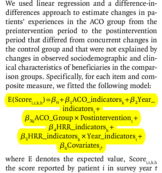
This example, taken from McWilliams et al. (2014), is much more typical of the kinds of regression models we see in applied settings. Without going into unnecessary detail on this paper’s background, the covariate called “ACO_indicators” is the treatment variable. The covariate \(\beta_{3k}\) represents the causal effect of interest. However, there are many other terms in the model, including time fixed effects, other fixed effects (“HRR_indicators”), and covariates. We talk about the inclusion of fixed effects below, followed by a discussion on adjusting for covariates using regression models.
Fixed effects in diff-in-diff
Let’s talk about fixed effects briefly (see Mummolo and Peterson (2018) for a more in-depth discussion of fixed effects models and their interpretation). Fixed effects, particularly unit-level fixed effects, are used in causal inference to adjust for unmeasured time-invariant confounders. Of course, there are trade-offs. The discussion from Imai and Kim (2019) explains that using unit fixed effects comes at the cost of capturing the dynamic relationship between the treatment and the outcome.
Kropko and Kubinec (2020) discuss the common two-way fixed effects model, which includes unit and time fixed effects. Their main point is that estimates coming from two-way fixed effect models are difficult to interpret when we have many time periods. When we have the canonical (two-period, binary treatment) diff-in-diff setup, the \(\beta\) coefficient from the two-way fixed effect model \(\left(y_{it} = \alpha_i + \delta_t + \beta D_{it} + \epsilon_{it}\right)\) equals the usual estimate. As more time periods are added within the fixed-effects framework, we implicitly add supplementary assumptions. In particular, the diff-in-diff effect is assumed homogenous across time and cases. Homogeneity across time is a stringent assumption that says the diff-in-diff effect is the same no matter how close or far apart the time periods are. We say this not to discourage use of two-way fixed effect models, but to discourage automatic use of them. True they work well for some cases (when we need to adjust for unmeasured time-invariant confounders), but we really need to examine our research goals on an application-by-application basis, consider the assumptions implicit in the models we’re thinking of using, and adjust our tools accordingly.
What if treated units are treated at different times? Goodman-Bacon (2021) examines the two-way fixed effect regression model \((Y_i(t) = \alpha_i + \delta_t + \beta D_{it} + \epsilon_{it})\) as a diff-in-diffs estimator when there exists treatment variation. It turns out that the TWFE estimator is a weighted combination of all possible \(2 \times 2\) diff-in-diff estimators found in the data. For example, consider three groups: an untreated group, an early-treated group and a late-treated group. The \(2 \times 2\) diff-in-diff estimators consist of three \(2 \times 2\) comparisons:
- Early-treated and late-treated groups vs. Untreated group in all periods
- Early-treated group vs. late-treated group in periods before late-group is treated
- Late treated group and early treated group in periods after early-group is treated
The weights of these \(2 \times 2\) estimators are based on the sample size in each group and the variance of the treatment variable. Note that the variance of a binary random variable is its expected value multiplied by \(1\) minus its expected value. Therefore, the variance of the treatment variable is decreasing in its expected value’s distance from \(0.5\). The implication, then, is that \(2 \times 2\) comparisons of groups that are closer in size and occur in the middle of the time window will receive the greatest weights.
In this setting with variation in treatment timing, Goodman-Bacon (2021) defines the variance-weighted ATT estimand as follows: In each of the three \(2 \times 2\) comparisons above, there is an ATT for the treated group in each of that comparison’s post-treatment periods. The variance-weighted ATT estimand calculates the average ATT over all post-treatment periods in each \(2 \times 2\) comparison and then sums the average ATT over all \(2 \times 2\) comparisons with weights equal to the probability limits of the estimators’ weights described above. So long as each timing group’s ATTs do not vary over time, Goodman-Bacon (2021) shows that a variance-weighted common trends assumption suffices for identification of the variance-weighted ATT. Moreover, when effects are constant both over time and units, the variance-weighted ATT is equal to the overall ATT, which makes the variance-weighted ATT estimand easier to interpret.
Bai (2009) describes an interactive fixed effects model that incorporates time-varying dynamics. Each unit is assumed to have an \(r\)-vector of factor loadings, \(\mathbf{\lambda}_i\), multiplies an \(r\)-vector of common factors at each time point \(\mathbf{F}_{t}\). That is, for outcome \(Y_{it}\) of unit \(i\) at time \(t\), the data-generating model is \[ Y_{it} = X_{it}'\beta + \lambda_{i1}F_{1t} + \ldots + \lambda_{ir}F_{rt} + \epsilon_{it}\;, \] where \(X_{it}\) are observed covariates. Note that the two-way fixed effects model is a special case of this where \(F_{1t} = 1\), \(F_{2t} = \delta_t\) and \(\lambda_{i1}= \alpha_{i}\), \(\lambda_{i2} = 1\). The authors present least-squares estimators for large \(N\) and large \(T\).
Marginal structural models can capture dynamics such as past outcomes affecting future treatments, but cannot account for time-invariant unmeasured confounders. Thus, we can either adjust for time-invariant unmeasured confounders and assume no dynamic relationship between treatment and outcome or we can assume that there are no unmeasured confounders and allow for more complicated relationships between treatment and outcome.
Confounding in linear settings
If we know how confounding arises, we can address it. For example, if the truth is a linear data-generating model, we can use a linear regression model to address confounding. The flowchart below outlines six linear data-generating models and the appropriate linear regression adjustment for each.
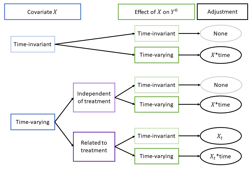
Of these six scenarios, two require no adjustment at all. Of the 4 that require adjustment, only one requires the regression adjustment type nearly always found in the literature, i.e., adjusting for a time-varying covariates without any interaction with time. In the other three scenarios with confounding bias, the issue is due, in whole or in part, to time-varying covariate effects. For these cases, including an interaction of covariates with time is crucial to addressing confounding bias.
See directed acyclic graphs (DAGs) (together with a brief discussion) for these scenarios by selecting an option below: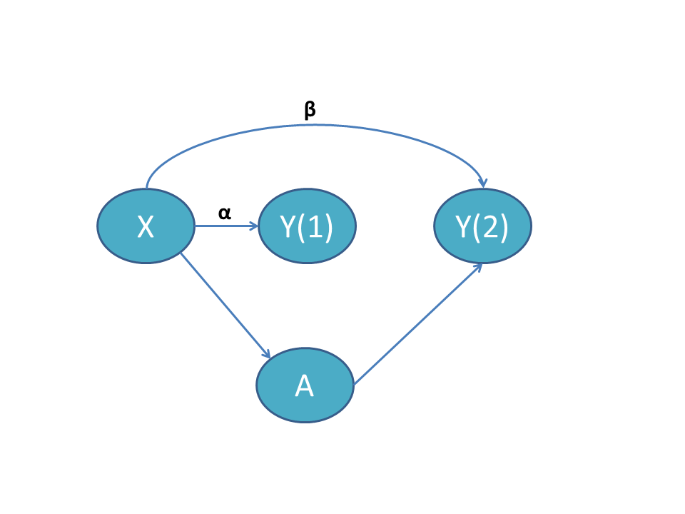
Time-invariant X with time-varying effect
In this scenario, the covariate \(X\) does not vary over time. The arrow from \(X\) to \(A\) indicates that \(X\) is a cause of \(A\), satisfying the first requirement of a confounder. Additionally, are arrows from \(X\) to \(Y(1)\) and to \(Y(2)\) as well as an arrow from \(A\) to \(Y(2)\). [Note: there is no arrow from \(A\) to \(Y(1)\) because treatment is administered after \(Y(1)\).] \(\alpha\) is the effect of \(X\) on \(Y(1)\), and \(\beta\) is the effect of \(X\) on \(Y(2)\). When \(\alpha = \beta\), the effect of \(X\) is time-invariant and we do not require covariate adjustment. When \(\alpha \neq \beta\), we must adjust for the interaction of \(X\) with time.
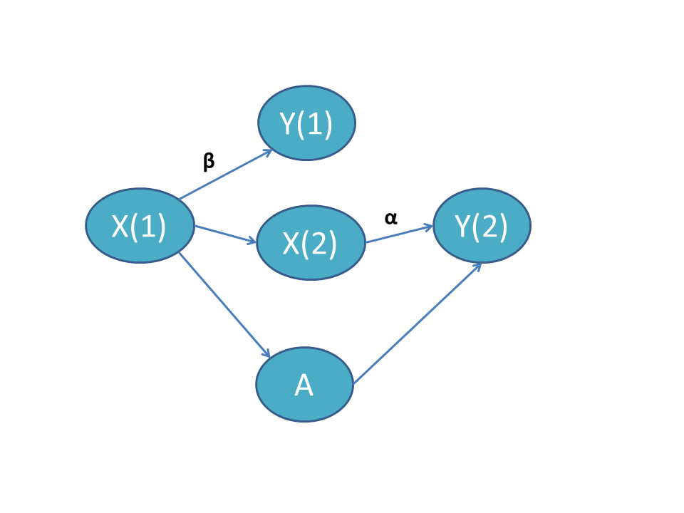
Time-varying X independent of treatment
In this scenario, the time-varying covariate \(X\) in periods 1 and 2 is denoted \(X(1)\) and \(X(2)\). There is no arrow connecting \(A\) to \(X(2)\), indicating that treatment does not affect the evolution of \(X(1)\) to \(X(2)\). When \(\alpha = \beta\), the effect of \(X\) is time-invariant and we do not need to adjust for the covariate. When \(\alpha \neq \beta\), we must adjust for the interaction of \(X\) with time.

Time-varying X related to treatment
In this scenario, the time-varying covariate \(X\) evolves differentially by treatment group. However, most diff-in-diff analyses implicitly or explicitly assume that \(X\) does not evolve based on treatment group. See our nonparametric section below. One diff-in-diff estimator that directly accounts for this phenomenon is Stuart et al. (2014), which we discuss in more detail below. When \(\alpha = \beta\), the effect of \(X_t\) on \(Y^0\) is time-invariant and it suffices to adjust only for \(X_t\). When \(\alpha \neq \beta\), we must adjust for the interaction of \(X_t\) with time.
Matching
Matching estimators adjust for confounding by balancing the treatment groups on measured covariates. Rather than using the entire sample population to estimate the diff-in-diff effect, units in the control group are selected by on their “closeness” to units in the treated group. We introduce this section by a series of tweets about a recent Daw and Hatfield (2018a) paper on matching and regression to the mean.
Do you use diff-in-diff? Then this thread is for you.
— Laura A. Hatfield, PhD (@laura_tastic) July 27, 2018
You’re no dummy. You already know diverging trends in the pre-period can bias your results.
But I’m here to tell you about a TOTALLY DIFFERENT, SUPER SNEAKY kind of bias.
Friends, let’s talk regression to the mean. (1/N) pic.twitter.com/M2tEEsBiyH
The argument focuses on estimators that match on outcomes in the pre-treatment period. Matching on pre-treatment outcomes is attractive in diff-in-diff because it improves comparability of the groups and possibly of their outcome trends. The crux of the argument in Daw and Hatfield (2018a) is that matching estimators can be dangerous in diff-in-diff settings due to regression to the mean. Regression to the mean is a notorious phenomenon in which extreme values tend to revert to the group mean on subsequent measurements. For example, if we select the ten students who score highest on an exam, at a subsequent exam, the average score for these ten students would drop towards the class mean.
For diff-in-diff, the effect is similar. By constraining the pre-treatment outcomes to be similar, we are more likely to select units of the group that are higher or lower than their respective group means. Once the matching constraint is dropped (in the post-treatment period), these units’ means can revert back to their respective group’s mean and possibly yield a spurious diff-in-diff effect. So in some cases, matching can actually introduce bias.
So how can we know whether matching is useful or harmful in our diff-in-diff study? Unfortunately sometimes we can’t know. Take the paper Ryan, Burgess, and Dimick (2015) which presents a simulation study using matching estimators and shows that matching can reduce confounding bias. In their paper, they sampled the treated and control groups from the same population, but the probability of being part of the treated group increased for high pre-treatment outcomes. In contrast, Daw and Hatfield (2018a) set up similar simulations but with treated and controls groups coming from different, but overlapping, populations.
For the following thought experiment, assume no diff-in-diff effect is present. If the populations are drawn as in Ryan, Burgess, and Dimick (2015), the two populations have different pre-treatment means. In a diff-in-diff study without matching, these units will regress to the mean in the post-treatment period (but they will regress to the same value since they are drawn from the same population!). This yields a non-zero diff-in-diff effect. Matching actually fixes this issue. If the populations are drawn as in Daw and Hatfield (2018a), the opposite is true. Without matching, the populations are different in the pre-intervention period and remain that way in the post-intervention period (since they are representative of their true populations, there is no regression to the mean). With matching, the populations are constrained to be the same in the pre-treatment period, and once the constraint is released in the post period, the two groups regress back to their group means. So in the Ryan, Burgess, and Dimick (2015) setup, matching is the solution to regression to the mean bias; in the Daw and Hatfield setup, matching is the cause of the regression to the mean bias.
Using real life data, there is no way to check empirically whether our groups come from the same population or from different populations. Determining this must come from expert knowledge from how the treatment assignment mechanisms work. To quote Daw and Hatfield (2018b) in the follow-up to their own paper:
(R)esearchers must carefully think through the possible treatment assignment mechanisms that may be operating in the real-life situation they are investigating. For example, if researchers are aware that a pay-for-performance incentive was assigned to physicians within a state based on average per-patient spending in the past year, one may be comfortable assuming that treatment assignment mechanism is operating at the unit level (i.e., the potential treatment and control units are from the same population). In contrast, if the same incentive was assigned to all physicians within a state and a researcher chooses a control state based on geographic proximity, it may be more reasonable to assume that treatment assignment is operating at the population level (i.e., the potential treatment and control units are from separate populations).
Other researchers have also noted the lurking biasedness of some matching diff-in-diff estimators. Lindner and McConnell (2019), for example, found that biasedness of the estimator was correlated in simulations with the standard deviation of the error term. As the standard error increased, so did the bias.
In a pair of papers, Chabé-Ferret (Chabé-Ferret 2015, 2017) similarly concluded that matching on pre-treatment outcomes can be problematic and is dominated by symmetric diff-in-diff.
Semi- and Non-parametric
Up to this point, we can think of a diff-in-diff analysis as a four-step process:
- make assumptions about how our data were generated
- suggest a sensible model for the untreated outcomes
- connect the untreated outcomes to the observed outcomes
- estimate the diff-in-diff parameter (via regression or matching or both)
While this process is simple, our estimates and inference can crumble if we’re wrong at any step along the way. We’ve discussed the importance of counterfactual assumptions and inferential procedures. We now turn our attention to the modeling aspect of diff-in-diff. So far, we have discussed only parametric models. Below, we present some semiparametric and nonparametric estimators for diff-in-diff. These give us more flexibility when we don’t believe in linearity in the regression model or fixed unit effects.
Semi-parametric estimation with baseline covariates
Abadie (2005) addresses diff-in-diff when a pre-treatment covariate differs by treatment status and also affects the dynamics of the outcome variable. In our confounding section above, this is the “Time-invariant X with time-varying effect” scenario.
Let’s return to the two-period setting. When a covariate \(X\) is associated with both treatment \(A\) and changes in the outcome \(Y\), the Counterfactual Assumption 1 no longer holds.
Thus, Abadie (2005) specifies an identifying assumption that conditions on \(X\). That is,
Conditional Counterfactual Assumption \[ \mathbb{E}\left[Y^0(2) - Y^0(1) \mid A = 1, X\right] = \mathbb{E}\left[Y^0(2) - Y^0(1) \mid A = 0, X\right]. \]
This assumption does not identify the ATT, but it can identify the CATT, that is, the conditional ATT:
Conditional average effect of treatment on the treated (CATT) \[ CATT \equiv \mathbb{E}\left[Y^1(2) - Y^0(2) \mid A = 1, X\right]. \]
The CATT itself may be of interest, or we may want to average the CATT over the distribution of \(X\) to get back the ATT. To identify the CATT, repeat the identification steps above with expectations conditional on \(X\). As expected, it turns out that
\[\begin{align*} \mathbb{E}\left[Y^1(2) - Y^0(2) \mid A = 1, X\right] &= \lbrace \mathbb{E}\left[Y(2) \mid A = 1, X\right] - \mathbb{E}\left[Y(1) \mid A = 1, X \right] \rbrace - \\ & \ \ \ \ \ \lbrace \mathbb{E}\left[Y(2) \mid A = 0, X\right] - \mathbb{E}\left[Y(1) \mid A = 0, X \right] \rbrace. \end{align*}\]
Nonparametric estimators for these quantities are easy when \(X\) is a single categorical variable. They are simply sample averages for groups defined by combinations of \(X\) and \(A\):
- The post-treatment average of the treated group with \(X=x\) for \(\mathbb{E}\left[Y(2) \mid A = 1, X=x\right]\)
- The pre-treatment average of the treated group with \(X=x\) for \(\mathbb{E}\left[Y(1) \mid A = 1, X=x\right]\)
- The post-treatment average of the control group with \(X=x\) for \(\mathbb{E}\left[Y(2) \mid A = 0, X=x\right]\)
- The pre-treatment average of the control group with \(X=x\) for \(\mathbb{E}\left[Y(1) \mid A = 0, X=x\right]\)
However, if \(X\) is high-dimensional or contains continuous covariates, these get tricky. Abadie proposes a semiparametric solution using propensity scores. Recall that a propensity score is the estimated probability of treatment given pre-treatment covariate \(X\), \(P(A = 1 \mid X)\). For this approach to work, we need to use the positivity assumption, which was introduced in the assumption section. That is,
Positivity Assumption \[\begin{equation*} 0 < P(A = 1 | X) < 1 \; \text{ for all } X. \end{equation*}\]
This assumption ensures the estimand is defined at all \(X\). If some values of \(X\) lead to guaranteed treatment or control (i.e., propensity scores of \(0\) or \(1\)) we should reconsider the study population.
With positivity in hand, consider the weighted estimator of Abadie (2005):
\[\begin{equation} \mathbb{E}\left[Y^1(2) - Y^0(2) \mid A = 1\right] = \mathbb{E}\left[\frac{Y(2) - Y(1)}{P(A = 1)} \cdot \frac{A - P(A = 1 \mid X)}{1 - P(A = 1 \mid X)}\right]. \end{equation}\]
To estimate these quantities, we need fitted values of the propensity scores for each unit, i.e., \(\hat{P}(A=1 | X= x_i)\) and then we use sample averages in the treated and control groups. To see the math,
We only need the average change in outcomes among the treated units and the weighted average change in outcomes among the control units. The weights are \(\frac{\hat{P}(A=1 | X=x_i)}{1 - \hat{P}(A=1 | X=x_i)}\). What are these weights sensible? Well, outcome changes among control units with \(x_i\) that resemble treated units (i.e., with large \(\hat{P}(A=1 | X=x_i)\)) will get more weight. Outcome changes among control units with \(x_i\) that resemble control units will get less weight.
To model the propensity scores, we could use a parametric model like logistic regression or something more flexible like machine learning. As usual, extending the model to multiple time points in the pre- and post-treatment periods is more complicated.
Nonparametric estimation with empirical distributions
Athey and Imbens (2006) developed a generalization of diff-in-diff called “changes-in-changes” (of which diff-in-diff is a special case). This method drops many of the parametric assumptions of diff-in-diff and allows both time and treatment effects to vary across individuals. Again we are in a two-period, two-group setting. The Athey and Imbens (2006) model is much less restrictive than the usual parametric model. It only assumes two things:
- \(Y_i^0 = h(u_i, t)\) for unobservable characteristics \(u_i\) and an unknown function \(h\) (increasing in \(u\))
- Within groups, the distribution of \(u_i\) does not change over time
Note that the distribution of \(u_i\) can differ between treatment groups so long as this difference remains constant. Below, we discuss a method for estimating diff-in-diff without this assumption. To estimate the target parameter, Athey and Imbens (2006) estimate empirical outcome distributions in a familiar list of samples:
- The post-treatment distribution of \(Y\) in the treated group,
- The pre-treatment distribution of \(Y\) in the treated group,
- The post-treatment distribution of \(Y\) in the control group, and
- The pre-treatment distribution of \(Y\) in the control group.
What we are missing is
- The post-treatment distribution of \(Y^0\) in the treated group (i.e., counterfactual, untreated outcomes)
Since we cannot observe this distribution, Athey and Imbens (2006) estimate it through a combination of the empirical distributions for (1), (2), and (3). After estimating (5), the effect of treatment is the difference between observed (4) and estimated (5). Let \(F_{Y^0_{12}}\) be the counterfactual distribution for the untreated outcomes for the treated group at \(t = 2\). We estimate this quantity through the relation:
\[ F_{Y^0_{12}}(y) = F_{Y_{11}}(F^{-1}_{Y_{01}}(F_{Y_{02}}(y)))\;, \] where \(F_{Y_{11}}\) is the distribution function for the (observed) outcomes for the treated group at \(t = 1\); \(F_{Y_{01}}\) is the distribution function for the (observed) outcomes for the untreated group at \(t = 1\); and \(F_{Y_{02}}\) is the distribution function for the (observed) outcomes for the untreated group at \(t = 2\).
The other distribution of note, \(F_{Y^1_{12}}(y)\), is actually observed since this are the treated outcomes for the treated group at \(t = 2\). Since we have estimates for both \(F_{Y^1_{12}}\) and \(F_{Y^0_{12}}\), we can also estimate the diff-in-diff effect. MATLAB code for this estimator is available on the author’s website.
Bonhomme and Sauder (2011) extend this idea to allow the shape of the outcome distributions to differ in the pre- and post-intervention periods. The cost of this additional flexibility is that they must assume additivity.
Semiparametric estimation with time-varying covariates
One of the key identifying assumptions from Athey and Imbens (2006) is that the distribution of \(u\) — all non-treatment and non-time factors — is invariant across time within the treated and control groups. That is, the distributions do not change with time. Stuart et al. (2014) circumvents this restriction by considering four distinct groups (control/pre-treatment, control/post-treatment, treated/pre-treatment, treated/post-treatment) rather than just two groups (control and treated) observed in two time periods. With the four groups, the distribution of \(u\) can change over time. A consequence of this setup is that it no longer makes sense to talk about the diff-in-diff parameter as the effect of treatment on the treated; instead, the estimand is defined as the effect of treatment on treated in pre-treatment period.
The estimator uses propensity scores for predicting the probabilities of each observation being in each of the four groups. We can use some kind of multinomial regression. The treatment effect is then calculated as a weighted average of the observed outcomes (see section 2.4 of Stuart et al. (2014)).
Double Robustness
Whereas standard parametric techniques rely on estimation of the outcome regression, and methods such as those in Abadie (2005) leverage information in the propensity score function, some doubly robust methods use both of these components. Broadly, doubly robust methods will yield unbiased estimates if one of these regressions is estimated consistently, and they will yield efficient estimates if both are estimated consistently.
Sant’Anna and Zhao (2020) propose a doubly robust estimator that allows for linear and nonlinear specifications of the outcome regression and propensity score function for panel or repeated cross-section data. Inference yielding simultaneous confidence intervals involves a bootstrapping procedure, which accommodates clusters (although the number of groups must be large).
Li and Li (2019) develop a doubly robust procedure specific to diff-in-diff, with an application to data about automobile crashes before and after the implementation of rumble strips. They parameterize the treatment effect using both multiplicative and additive quantities
Elsewhere, Han, Yu, and Friedberg (2017) implement a double robust weighting approach based on Lunceford and Davidian (2004) to study the impact of medical home status on children’s healthcare outcomes. General texts on double robust estimators are available (see van der Laan and Robins (2003) or van der Laan and Rose (2011)). For another type of doubly robust method that depends on the outcome regression and unit and time weights, see Arkhangelsky et al. (2021) in the Synthetic Control section.
Inference
Inference and estimation are closely linked. Once we estimate the causal estimand, we want to know how uncertain our estimate is and test hypotheses about it. In this section, we highlight some common challenges and proposed solutions for inference in diff-in-diff.
Whether the data arise from repeated measures or from repeated cross-sections, data used in diff-in-diff studies are usually not iid (i.e., independently and identically distributed). For example, we often have hierarchical data, in which individual observations are nested within larger units (e.g., individuals in a US state) or longitudinal data, in which repeated measures are obtained for units. In both of these cases, assuming iid data will result in standard errors that are too small.
Below, we discuss three common issues in inference: serial autocorrelation, clustered data, and distributional assumptions. We draw on three papers in this area: Bertrand, Duflo, and Mullainathan (2004), Rokicki et al. (2018), and Schell, Griffin, and Morral (2018).
Collapsing the data
Collapsing the data by averaging the pre- and post-intervention observations returns us to the simple two-period setting, obviating the need to consider longitudinal correlation in the data. When treatment is administered at the same time point in all treated units, we can perform ordinary least squares on the aggregated data. On the other hand when treatment is staggered (e.g., states pass the same health care law in different years), Bertrand, Duflo, and Mullainathan (2004) suggest aggregating the residuals from a regression model and then analyzing those. See Goodman-Bacon (2021) and Athey and Imbens (2022) for more about varying treatment times.
In simulation studies, Bertrand, Duflo, and Mullainathan (2004) and Rokicki et al. (2018) find that aggregation has good Type I error and coverage, but it does lose some information (and thus power).
Clustered and robust standard errors
The most popular way to account for clustered data in diff-in-diff is clustered standard errors (Cameron and Miller 2015; Abadie et al. 2023). This adjusts the usual variance-covariance matrix estimate by accounting for correlation in the data. In Stata, this is as simple as using the cluster option in the regress function. In R, the vcovHC package implements a huge variety of alternative variance-covariance methods.
However, clustered standard error methods fail with only one treated unit (Conley and Taber 2011), for example, when a single state implements a policy of interest. There is no hard and fast rule on the number of treated units needed for clustered standard errors to be appropriate. Figures 2 (panel A) and 4 of Rokicki et al. (2018) show that when the number of groups is small, clustering standard errors results in under-coverage, which gets worse as the treated-to-control ratio becomes more unbalanced.
Donald and Lang (2007) developed a two-part procedure for estimation and inference in simple models that works well even when the numbers of groups is small.
Mixed models with random effects at the cluster level can account for serial correlation. This is what we used in our demonstration of confounding in a previous section.
Robust standard errors estimation methods (aka sandwich estimators or Huber-White) are meant to protect against departures from the assumed distributional form of the errors. However Schell, Griffin, and Morral (2018) found that across a range of simulations, these robust standard error estimates were worse than no adjustment or other methods of adjusting standard errors. They caution (p 36), “researchers should be quite cautious about using so-called robust SEs with longitudinal data such as these.”
Generalized estimating equations
Generalized estimating equations (GEE) take into account covariance structure and use a robust sandwich estimator for the standard errors (see Figure 2, panel D and Figure 4 in Rokicki et al. (2018)). Both of these methods are widely available in statistical software. In particular, GEE is powerful since it is robust to misspecification of the correlation structure. Specifying the correct covariance will increase the efficiency of the estimate. However, note that Rokicki et al. (2018) also found under-coverage in the confidence interval in the GEE estimates when the ratio of treated to control units was lopsided.
Arbitrary covariance structures
Throughout the diff-in-diff literature, we find simulations and inference techniques based on an autoregressive covariance AR(1) structure for the residuals within a cluster. The AR(1) covariance structure is
\[ \text{Cov}(Y_i) = \sigma^2 \begin{pmatrix} 1 & \rho & \rho^2 & \cdots & \rho^{n-1} \\ \rho & 1 & \rho & \cdots & \rho^{n-2} \\ \rho^2 & \rho & 1 & \cdots & \rho^{n-3}\\ \vdots & \vdots & \vdots & \ddots & \vdots \\ \rho^{n-1} & \rho^{n-2} & \rho^{n-3} & \cdots & 1 \end{pmatrix} \]
with an unknown variance parameter \(\sigma^2\) and an unknown autoregressive parameter \(0 \leq \rho \leq 1\). When \(\rho\) is larger, clustered values are more highly correlated; whereas when \(\rho = 0\), observations are independent. This structure assumes that correlation is positive (or zero) across all observations and that observations closer to each other are the most strongly correlated, and observations that are more distant are more weakly correlated.
An assumed AR(1) correlation structure is common in diff-in-diff simulation studies and inference techniques. Bertrand, Duflo, and Mullainathan (2004) considered this correlation structure in simulations and found that “this technique [assuming AR(1)] does little to solve the serial correlation problem” due to the difficulty in estimating \(\rho\). Rokicki et al. (2018) used an AR(1) in their simulations. As we illustrate in the app below, with unit and time fixed effects, AR(1) is not a plausible correlation structure.
McKenzie (2012) also discusses autocorrelation, emphasizing how statistical power relates to the number of time points and to autocorrelation, ultimately concluding that ANCOVA is more powerful than diff-in-diff.
The correlation structure in diff-in-diff applications may follow many different structures. For example, after de-meaning and de-trending, outcomes have a weak positive correlation in adjacent time points but a negative correlation at time points in far apart time points. In the shiny app below, we present correlation structures for simulated data and real data. The real datasets are from (a) the Dartmouth Health Atlas, (b) MarketScan claims data, and (c) Medicare claims, which are described in more detail within the app. Play around with the settings to simulate data that look like your applications. Does the correlation structure look the way you expect?
Permutation tests
Permutation tests are a resampling method that can be used to test statistical hypotheses. In the diff-in-diff setting, permutation tests comprise the following steps:
Compute the test statistic of interest on the original data. For example, calculate the interaction term between time and treatment from a regression model. Call this \(\hat{\delta}\).
For \(K\) a large positive integer, permute the treatment assignment randomly to the original data, so that the data are the same save for a new treatment assignment. Do this \(K\) times.
For each of the \(K\) new datasets, compute the same test statistic. In our example, we compute a new interaction term from a regression model. Call these \(\hat{\delta}^{(k)}\) for permutation \(k \in \{1, \dots, K\}\).
Compare the test statistic \(\hat{\delta}\) found in the first step to the test statistics \(\hat{\delta}^{(1)}, \dots, \hat{\delta}^{(K)}\) found in the third step.
The fourth step is where we can get a nonparametric p-value for the parameter of interest. If, for instance, \(\hat{\delta}\) is more extreme than 95% of \(\hat{\delta}^{(k)}\) then the permutation test p-value is 0.05.
For more on permutation inference for difference-in-differences, see Conley and Taber (2011) and MacKinnon and Webb (2020).
Lagged dependent variable regression
A promising technique to address serial autocorrelation is to include lagged variables. (Schell, Griffin, and Morral 2018) The form of the regression model is different from the specifications above, since it uses change coding of the treatment indicator and includes the previous time-period’s value of the outcome as a regressor: \[ Y_i(t) = \beta (D_{it} - D_{i,t-1}) + \gamma Y_i(t-1) + \alpha_i + \delta_t + \epsilon_{it} \]
In simulations, these authors show dramatic impacts on Type I error rates from inclusion of lagged dependent variables with change coding.
Design-based Inference
We usually conceptualize Difference-in-Differences designs in the framework of random sampling of treated and control units from a target population. Yet as Manski and Pepper (2018) and others point out, it can sometime be difficult to conceive units in a study as having been sampled from a larger population of units, e.g., when the units are all provinces in a particular country. In such settings, Rambachan and Roth (2022) propose a method of inference that treats random assignment of units to treatment and control as the stochastic process that generated the data. This finite population framework has the benefit of enabling inference when units in a study were not in fact sampled from a larger target population.
In this setting, the ATT (our usual causal target) is not a population quantity that is fixed over different possible random samples from this population. The ATT is a random quantity that changes over different possible random assignments depending upon which units happen to be assigned to treatment (Sekhon and Shem-Tov 2021). Hence, Rambachan and Roth (2022) define the ATT as the expected average effect among treated units, where the expectation is over the set of possible random assignments with unknown assignment probabilities.
Ideally, in a finite population setting, the researcher knows the true probabilities with which units could have wound up in treatment and control conditions. In the absence of a randomized experiment, though, we do not know these probabilities. Instead, Rambachan and Roth (2022) invoke an alternative assumption: The covariance of control potential outcomes and units’ treatment assignment probabilities is \(0\). This assumption will be satisfied in a randomized experiment since all units have the same treatment assignment probabilities. However, this assumption can also be satisfied when treatment assignment probabilities are not constant and control potential outcomes differ across units with different treatment assignment probabilities. The key condition is that control potential outcome do not linearly depend on treatment assignment probabilities; nonlinear dependence is okay.
In a panel setting with outcomes measured over time, Rambachan and Roth (2022) show that the assumption of linear independence between control potential outcomes and assignment probabilities is a finite population analogue of the standard parallel trends assumption: The assumption implies that the after-minus-before mean of the treated group’s control potential outcomes is equal, in expectation over possible random assignments, to the after-minus-before mean in the control group’s control potential outcomes. When this condition is satisfied, the after-minus-before mean of the treated group’s treated potential outcomes minus the after-minus-before mean in the control group’s control potential outcomes is unbiased for the ATT. In addition, Rambachan and Roth (2022) derive (1) an upper bound for the estimator’s variance, (2) an unbiased estimator of this upper bound, and (3) establish the asymptotic Normality of the estimator. Taken all together, the method in Rambachan and Roth (2022) enables us to do design-based inference for DID without having to assume that our study is equivalent to a randomized experiment.
Robustness
In this section, we summarize robustness checks relevant to diff-in-diff. We’ve highlighted diff-in-diff’s reliance on strong, untestable causal assumptions and discussed common estimation and inference methods. Many things can go wrong — assumptions don’t hold, wrong modelling choices, etc. We discuss a few techniques here that can help us quantify the robustness of our diff-in-diff estimates.
Placebo Tests
Lechner (2011) perform a thought experiment that we summarize here. Imagine we are doing a data analysis using diff-in-diff, and that our data have multiple pre-treatment time points. Now, imagine we move the “treatment time” to time before the real treatment. If we conduct a diff-in-diff analysis, what would you expect the estimated treatment effect to be? Perhaps you would expect no treatment effect, since no treatment occurred at that time. This idea underlies the use of placebo tests as a sensitivity check for diff-in-diff studies. Slusky (2017) use this technique to show that significant changes in health insurance coverage among people aged 19-25 (who were affected by the ACA’s dependent coverage provision) relative to those 16-18 or 27-29 (two possible comparison groups) occurred at several time points before the ACA was implemented.
Instrumental Variable Approach For Diverging Trends
Freyaldenhoven, Hansen, and Shapiro (2019) propose an approach to address the issue of diverging parallel trends due to an unobserved confounder. Their approach identifies an observed covariate that serves as an instrument for the unobserved confounder. They assume there is a latent variable that triggers treatment once it passes a threshold. For example, once a person’s income falls below a particular threshold, she becomes eligible for food stamps. They show that if we can identify a covariate that is related to income but unrelated to the food stamp intervention, we can use 2-stage least squares to estimate an unbiased treatment effect. This method is appealing both because it provides a mechanism to address bias and encourages researchers to think explicitly about unobserved confounders and their role in inducing bias. However, this framework relies heavily on being able to identify and find an instrument for unobserved confounders, which may be difficult to do in practice.
Sensitivity Analysis
Rambachan and Roth (2022) develop inference for the situation when parallel trends may not hold exactly, but we can impose restrictions on the extent to which parallel trends is violated. To do this, Rambachan and Roth (2022) introduce an additional parameter — the post-treatment difference in trends between treated and control groups — and inference that is valid under a restriction about the set to which the value of this parameter belongs. They provide several intuitive ways for researchers to restrict the possible values of the post-treatment difference in trends. Two such restrictions are as follows:
Relative Magnitude: The post-treatment difference in trends is no greater than some magnitude, \(\bar{M}\), of the maximum pre-treatment difference in trends.
Smoothness: The change in the post-treatment difference in trends between consecutive periods is less than or equal to some \(M \geq 0\).
These two restrictions can be combined in useful ways, e.g., placing a bound on (a) the post-treatment change in the difference in trends between consecutive periods in terms of (b) some magnitude of the pre-treatment change in difference in trends between consecutive periods.
Given such restrictions, the unknown causal target could be any of a set of values consistent with the restriction on the difference in trends. Rambachan and Roth (2022) propose a method of inference that, under reasonable assumptions, achieves the following aim: Over these possible values for the causal target, the lowest possible coverage probability for a random confidence interval is at least \(1\) minus the size (\(\alpha\)-level) of the test. Rambachan and Roth (2022) also provide conditions that ensure the probability of rejecting causal parameter values inconsistent with the restriction tends to \(1\) as the sample size grows.
This inferential method also leads to a valuable form of sensitivity analysis: studying the behavior of inference under more or less lax restrictions on the post-treatment difference in trends. For example, consider increasingly lax restrictions in terms of the relative magnitude bound, \(\bar{M}\). When \(\bar{M} = 0\), parallel trends is true, and only one value of the causal target is consistent with this restriction. As \(\bar{M}\) increases, more values of the causal target will be consistent with the restrictions on the difference in trends. Consequently, confidence intervals will become wider. Researchers can then answer questions like: How large would the post-treatment deviation from the pre-treatment difference in trends need to be in order to make my confidence interval cross the null?
Nonlinear Models
Much of diff-in-diff theory and its applications focus on continuous outcomes, but nonlinear outcomes are common too. Nonlinear outcomes include binary outcomes such as death status or count outcomes such as the number of hospitalizations. If we have a binary outcome, we can model the probability directly with a linear probability model; the downside to this approach is that predicted probabilities can fall outside of the \([0, 1]\) range. We can restrict predicted probabilities within \([0, 1]\) using an appropriate transformation — logit and probit transformations are perhaps the most common. However, in doing so we lose a lot of nice properties that come with the linear model. Ai and Norton (2003) first pointed out this vexing occurrence with respect to to diff-in-diff. In particular, they showed that the cross-partial effect can be nonzero even when the treatment/post-period interaction term is 0.
Puhani (2012) noted that while the point from Ai and Norton (2003) is true, the true diff-in-diff estimate is still taken directly from the interaction term in the model. He shows that diff-in-diff is actually a difference of two cross-partial derivatives so the interaction term always has the same sign as the diff-in-diff effect (not necessarily the case in Ai and Norton (2003)). Thus, inference on the treatment effect can be conducted through the usual test of the interaction parameter.
The Karaca-Mandic, Norton, and Dowd (2012) paper ties the previous two papers together. They show in Figures 3 and 4 how the diff-in-diff effect (on the probability scale) can change as the value of the linear predictor \(X\beta\) changes, even when the model does not include an interaction term. The authors then go through an interactive example using Stata, which might be useful to researchers intending to do a diff-in-diff analysis with a nonlinear model.
Another tricky aspect of nonlinear models is that the role of covariates is more complex than described above.
e.g. In OLS, if you omit a variable that's correlated with your outcome but not the tx, you still have an unbiased estimate of your beta. In logistic regression, even covariates that are not correlated with treatment can act as confounders and bias your ORs!
— Alyssa Bilinski (@ambilinski) February 5, 2020
Synthetic controls
In selecting a comparison group of units not impacted by the intervention, a researcher has many options. For example, to evaluate the impact of the Massachusetts health insurance expansion, a researcher could use all other states as controls. She could use nearby states as controls. She could even choose counties from around the US that look similar to Massachusetts counties. When conducting DID, researchers often use subject matter knowledge to choose comparison groups and then evaluate whether trends are parallel.
The synthetic control methods is an appealing alternative because it is a data-driven way to select comparison groups. The first instance of the synthetic control method is taken from Abadie and Gardeazabal (2003), which studied effects of terrorism on economic growth in Spain. Beginning in the 1960s, the Basque Country experienced a rash of terrorism, which was broken by a 1998 cease-fire. The other regions of Spain were weighted to form a synthetic Basque Country, similar to the real Basque Country in demographics. The results showed that per capita GDP increased in Basque Country after the cease-fire relative to the synthetic Basque country with no cease-fire.
In the years since that original synthetic control paper, many methodological refinements and extensions have been published. We summarize some of these below, but first, we consider potential pitfalls of synthetic controls.
The assumption that a weighted set of comparison units can represent the treatment group’s counterfactual outcomes is strong, and if not met, can introduce bias. Modifications to add flexibility to SCM include allowing a level difference between the treatment and comparison groups or allowing weights that do not sum to 1 and are negative (Doudchenko and Imbens 2016). Another alternative to address the convex hull issue is to develop synthetic controls for comparison units rather than treatment units and include only those that are well-estimated in the effect estimate (Powell 2018).
Another potential issue with SCM is overfitting. Several authors have observed that under a fixed penalty, SCM is a form of ridge regression. They have, therefore, proposed choosing the SCM penalty term to minimize mean-squared error to avoid overfitting (Doudchenko and Imbens 2016; Kinn 2018). In an alternative approach, Powell (2018) modeled unit-specific trends to reduce noise.
A third concern is the ‘curse of dimensionality’ (Ferman and Pinto 2021). Traditional SCM are consistent as the number of time periods goes to infinity. However, an increasing number of time periods decrease the likelihood that appropriate weights exist; with more time periods, the treatment unit may not fall inside the convex hull of the comparison units. Ben-Michael, Feller, and Rothstein (2021) propose adjusting the SCM estimate by the outcome regression-estimated average difference between treatment and comparison units (including lagged outcomes and possibly covariates). We discuss their augmented synthetic control method in more detail below.
Finally, because synthetic controls weight on pre-period outcomes (and since weighting and matching are close cousins), one might wonder about regression to the mean bias (as discussed above). A working paper by Illenberger, Small, and Shaw (2020) uses simulation to show that the same issues that plague diff-in-diff with matching on pre-period outcomes also affect synthetic controls. As in diff-in-diff, the problem worsens with larger baseline differences between treated and control group means and decreases with the auto-correlation in the outcomes. Those authors propose a correction that subtracts off the portion of the treatment effect due to regression to the mean. By assuming various values of baseline means, auto-correlation, and residual variance parameters, researchers can understand what values would be sufficient to materially change their treatment effect estimates.
Ding and Li (2019) study the relationship between diff-in-diff and related methods that assume treatment assignment is ignorable conditional on past outcomes (which includes synthetic controls and lagged dependent variables regression). These authors extend results from linear models to nonparametric settings. Their results apply when two conditions hold: stationarity (i.e., the outcomes would not get infinitely large over time) and stochastic monotonicity (i.e., either treated or control has smaller lagged outcomes), both of which can be empirically checked. When stationarity holds and the treated group has smaller lagged outcomes, the diff-in-diff treatement effect will be greater than or equal to the lagged dependent variable effect, and vice versa.
Synthetic Difference-in-Differences
Arkhangelsky et al. (2021) propose an extension to SCM called Synthetic Difference-in-Differences (SDID), which combines elements of both DID and SCM. Most DIDs incorporate both unit and time fixed effects, which weights each comparison unit and each time period equally. SCM incorporate unit-level weights and time fixed effects. SDID adds additional flexibility by incorporating all of these elements: 1) unit and time fixed effects and 2) unit- and time-level weights.
\[ \hat{\omega}^{sc} = \underset{\omega \in W}{\text{arg min}} \sum^{T-1}_{t = 1} \left(\sum^{N-1}_{i=1} \omega_iY_i(t) - Y_N(t)\right)^2 \]
\[ \hat{\lambda}^{sc} = \underset{\lambda \in L}{\text{arg min}} \sum^{N-1}_{i = 1} \left(\sum^{T-1}_{t=1} \lambda_iY_i(t) - Y_i(T)\right)^2 \]
\[ \left(\hat{\theta}^{sdid}, \hat{\tau}^{sdid}\right) = \underset{\theta}{\text{arg min}} \sum^N_{i=1}\sum^T_{t=1}\left( Y_i(t) - g(\theta)_{it} - \tau W_{it}\right)^2\hat{\omega}_i\hat{\lambda}_t \]
The authors demonstrate that this approach is doubly-robust: as \(N\) and \(T\) go to infinity, the SDID estimators is consistent if either 1) the unit and time weights or 2) the outcome model are correctly specified. (This roughly corresponds to either SCM with additional weight flexibility or DID being consistently estimated.)
Augmented Synthetic Control
Augmented SCM (ASCM) is another extension of synthetic controls. Ben-Michael, Feller, and Rothstein (2021) select weights to minimize the difference in pre-intervention level then subtract an estimate of the remaining level difference from the post-intervention difference. This addresses the “curse of dimensionality”: while SCM is unbiased as the number of pre-intervention time periods grows, researchers are less likely to identify a good fit as the number of time periods grows, even when one exists, unless they have a very large number of control units. Both ASCM and SDID methods can weight up recent periods relative to distant periods when estimating this level difference. Further, both ASCM and SDID involve a correction to the SCM estimator that is 0 if there is exact pre-intervention balance. These methods only apply when there is imperfect pre-intervention balance and matter most when there is substantial pre-intervention imbalance.
Generalized Synthetic Control
Xu (2017) proposed the generalized synthetic control method, which combines an interactive fixed effects model with the framework of synthetic control. The basic idea is to use a parametric factor model for the outcomes to predict the “missing” untreated potential outcomes for the comparison group. The factor model assumes that a small set of time-varying factors interact with unit-specific “factor loadings” to generate the outcome. Note that the popular two-way fixed effects model (with unit and time fixed effect) is a special case of a factor model.
Within the generalized synthetic control framework, Xu (2017) writes the outcome for unit \(i\) at time \(t\) as
\[ Y_i(t) = \delta_{it}D_{it} + x_{it}\beta + \lambda_i f_t + \epsilon_{it}, \]
where \(D_{it}\) is a treatment indicator which equals 1 whenever the unit \(i\) receives treatment at time \(t\), \(\delta_{it}\) are heterogeneous effects, \(x_{it}\) and \(\beta\) are covariates and their coefficients, and \(\lambda_i\) and \(f_t\) are factor loadings and factors, respectively.
To use the generalized synthetic control method, we first estimate the latent factors, \(f_t\), and the coefficients on the covariates, \(\beta\), using only the data from the control units (with least squares and some additional restrictions like orthogonality of the factors). Then we estimate the factor loadings of each treated unit, \(\lambda_i\), by minimizing a least squares equation for the treated units’ outcomes in the pre-treatment period, conditional on the factors and coefficients estimated in the first step. Finally, we use the estimated coefficients, factors, and factor loadings in the parametric outcome model to predict counterfactual untreated outcomes in the post-treatment period for the treated units:
\[ \hat{Y}^0_i(t) = x_{it}\hat{\beta} + \hat{\lambda}\hat{f_t}. \]
Following this step, the ATT is simply the average (within the treated group only) of the observed post-treatment outcomes minus the predicted untreated outcomes:
\[ ATT(t) = \frac{1}{N_t} \sum_i Y_i(t) - \hat{Y}^0_i(t), \] where the summation iterates over all treated units and \(N_t\) denotes the number of treated units.
The strengths of the method are that the factor structure can address time-varying confounding (unlike diff-in-diff); it incorporates heterogeneous treatment effects (unlike interactive fixed effects); and it can accommodate multiple treated units, observed covariates, and treated units outside the convex hull of the controls (unlike the synthetic control formulation of Abadie, Diamond, and Hainmueller (2010)). The limitations of this method include the requirement for a reasonably long pre-treatment period, the reliance on a parametric model for the outcome, and the lack of obvious safeguards against inappropriate controls (i.e., those that lack common support with the treated units).
Comparative interrupted time series
A related technique (sometimes described as equivalent to diff-in-diff with multiple time points) is comparative interrupted time series (CITS). The causal assumptions of the two methods are different, however. In CITS, the counterfactual is constructed by 1) fitting linear models to the comparison group’s outcomes in the pre- and post-intervention periods, 2) computing the pre- to post-period changes in the intercepts and slopes, 3) fitting a linear model to the treated group’s outcomes in the pre-intervention period, and 4) assuming the comparison group’s intercept and slope changes computed in step 2) would have held in the treated group in the absence of intervention.
We highlight some important differences between DID and CITS:
- CITS does not require parallel outcome evolution in the treated and comparison groups in the pre-intervention period
- CITS does require a linear model to capture the pre- to post-intervention change in the outcome process of the comparison group (which is then assumed to also hold for the treated group’s counterfactual untreated outcomes)
Notice that these are not merely differences in modeling. They are differences in the construction of the counterfactual:
- DID assumes the pre-to-post change in the average outcomes of the comparison group would also have been observed in the treated group, absent the intervention.
- DID with a pre-period slope difference assumes the pre-to-post change in the average outcomes of the comparison group plus the linearly growing difference observed in the pre period would combine to produce the treated group’s counterfactual outcomes, absent the intervention.
- CITS assumes the pre-to-post change in the intercept and slope of the comparison group would have been observed in the treated group, absent the intervention.
Parallel paths
Up to this point, identifying the diff-in-diff estimator required parallel trends or some type of counterfactual assumption. Mora and Reggio (2012) and Mora and Reggio (2019) developed a diff-in-diff estimator using an alternative assumption called the parallel growth assumption. The parallel growth assumption essentially requires that the derivatives of the paths are parallel. For example, imagine we have two linear functions — \(f(x) = 2x\) and \(g(x) = 3x\). These functions are not parallel, but their derivatives, \(f'(x) = 2\) and \(g'(x) = 3\), are.
Imagine the following scenario with five time points in which treatment is administered after time 3. The trajectory of the untreated outcomes for the control group (all observed by the consistency assumption) are shown with the orange dotted-dashed line. The trajectory of the untreated outcomes for the treated (observed up to the 3rd time point) is shown in the blue solid line.
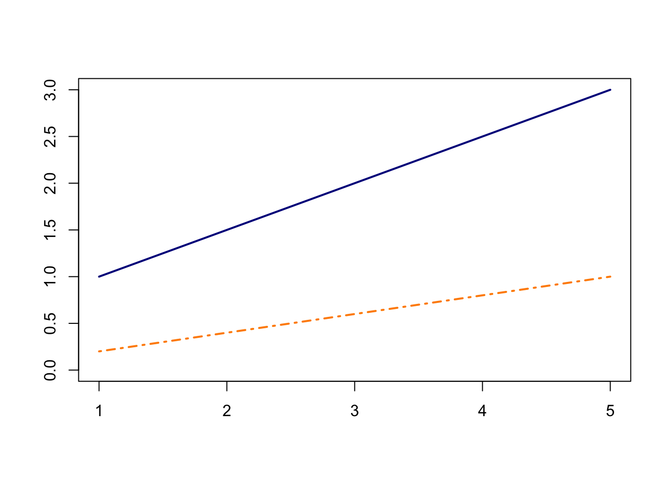
Clearly, this scenario violates the parallel trends assumption. In fact using parallel trends, the counterfactual untreated outcomes for the treated would deviate from their true trajectory shown by the dashed line below.
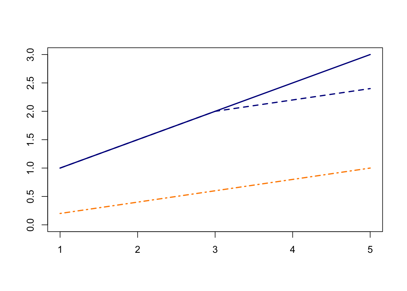
In this example any inference using diff-in-diff methods based on parallel trends will be biased. However, in this particular case, Mora and Reggio (2012) showed that the treatment effect is identified under an alternative assumption – parallel growth assumption. This assumption is similar to parallel trends except that we require the derivatives of the trajectories to be parallel. In the above graph, the two trajectories are not parallel, but their derivatives are! Both are straight lines with constant derivatives. Since the derivatives are parallel, the authors show that the estimator is identified. While interesting in theory, it is difficult enough justifying parallel trends using our original data (i.e., not derivatives or lagged differences), and it’s hard to imagine when we could be confident in parallel trends on the derivatives but not on the original scale. However, this paper is useful in understanding the role of the underlying diff-in-diff assumptions and which other assumptions may be possible to obtain similar quantities, especially in the case where parallel trends fails.
Multitask Gaussian processes
Ben-Michael et al. (2023) propose the use of multitask Gaussian processes (MTGPs) in a panel data setting. This approach models a unit’s untreated potential outcomes in time period \(t\) in terms of a model component plus a random error term with mean equal to \(0\). As the term Gaussian in the name of the method suggests, researchers conventionally suppose that untreated potential outcomes follow a multivariate Gaussian distribution. The model component is indexed by unit, \(i\), and time period, \(t\). Defined on the model components is a Gaussian process prior characterized by time and unit kernels. The role of the time kernel is to determine how the parameter values of the model in time \(t\) correlate with the model’s parameter values in later time periods. That is, the kernel captures how much information the model in one time period provides for the model in later time periods. At a high level, the unit kernel captures the correlation between untreated potential outcomes of any two distinct units, \(i\) and \(i^{\prime}\). Common kernels, such as the usual squared exponential kernel, are such that the correlation between model parameters is decreasing in the difference between any two time periods. This property is intuitively sensible in that information about potential outcomes in the year 1996 will probably contain more information about potential outcomes in 1997 than in 2023. Likewise, given a suitable (but perhaps less immediately apparent) definition of distance between two units, the untreated potential outcome of one unit provides less information about that of another unit the “further away” it is.
Estimation and inference proceed by updating the Gaussian process priors on the model parameters via a model-based likelihood function. With this prior distribution on the model parameters, researchers can then draw from the posterior distribution of the model parameters; input each draw as the parameters of the model of untreated potential outcomes; draw each of the treated units’ untreated potential outcomes; and then directly calculate the ATT from the treated units’ observed treated potential outcomes and their imputed control potential outcomes. Repeating this procedure many times will yield a simulation-based approximation to the posterior distribution of the ATT.
Two of the key benefits of the MTGP model are as follows. First, the functional form of the model component is nonparametric. Along these lines, Ben-Michael et al. (2023) show that the MTGP model’s posterior predictive mean can be represented as a weighting estimator (with weights for both time and units). While the mean squared error of this weighting estimator depends on the true, unknown functional form of the model component, Ben-Michael et al. (2023) show that the weights are effectively chosen to minimize the estimator’s worst-case, mean squared error over all functions in a large class of possible functions. Second, because of the time kernels, MTGP model has intuitive appeal in that uncertainty about ATTs will be greater for periods further away from the onset of treatment, which is a property that many existing methods of uncertainty quantification lack.
Acknowledgments
The bulk of this website was written and edited by Bret Zeldow, Thomas Leavitt and Laura Hatfield. Funding for this website was provided by the Laura and John Arnold Foundation. Additional content contributors are Alyssa Bilinski, Carrie Fry, and Sherri Rose. Many thanks to Savannah Bergquist, Austin Denteh, Alex McDowell, Arman Oganisian, Toyya Pujol-Mitchell, and Kathy Swartz for their helpful comments. This website is built using the R package blogdown and hosted on Netlify. The design is based on the Kraiklyn Hugo theme.
References
© 2019 Bret Zeldow and Laura Hatfield